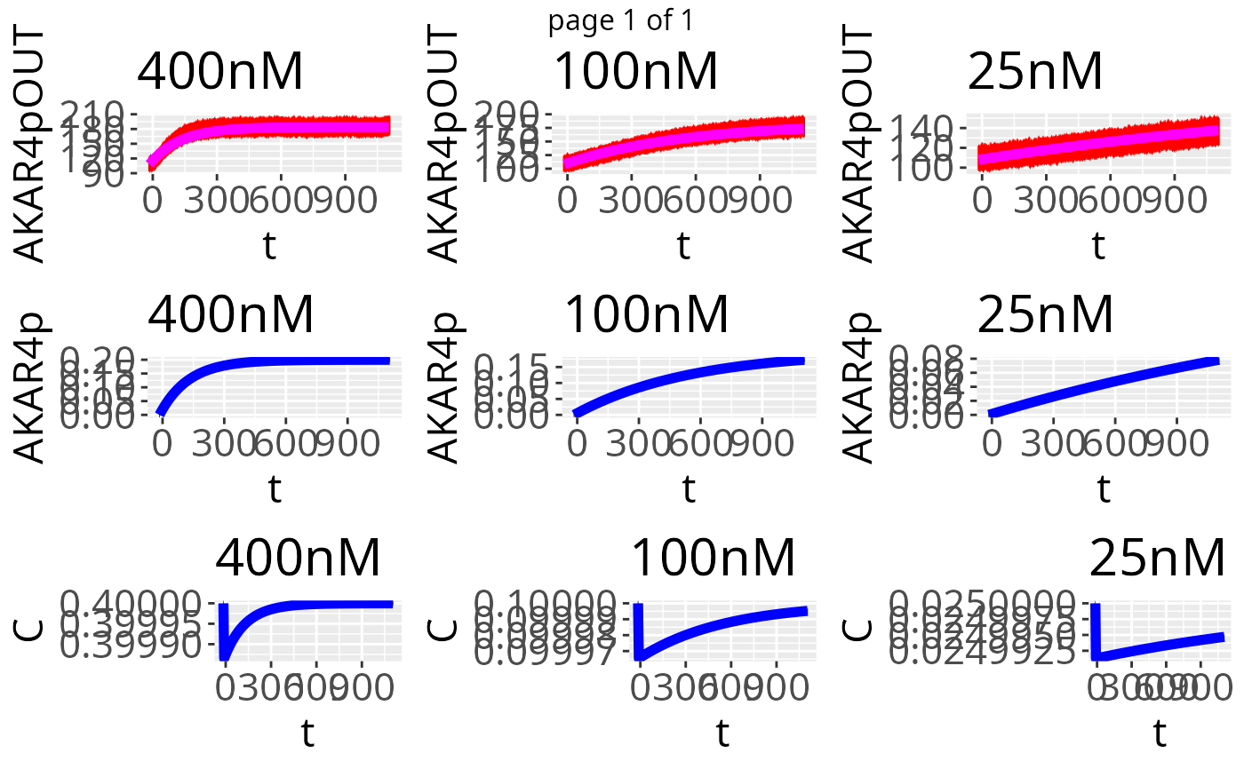
Plot time series simulation with state variables

This function plots simulations of time series experiments and plots them against experimental data. The input in the provided experiments must differ only in one vector component.

Usage

ggplot_time_series_states(
  simulations,
  experiments,
  var.names = NULL,
  type = "boxes",
  plot.states = TRUE,
  ttf = identity,
  xl = "t",
  yl.func = NULL,
  yl.state = NULL,
  MLE = 1
)

Arguments

simulations

list of simualtions as output from the simulator

experiments

list of experiments

var.names

override the rownames of the simulation results

type

'boxes' or 'lines'

plot.states

TRUE (or FALSE) - whether to plot the state variables or only the functions

ttf

time transformation function - the plot will be against ttf(t), where t is a vector of the experiment's output times, ttf can adjust the time vector if it is very uneven or requires other modification only when plotting, e.g. seq_along.

xl

x-axis label (time usually)

yl.func

y-axis-limits of function plots, can be a list of ggplot2::ylim() objects, with NULL elements for automatic mode (the neutral element), NA elements will trigger tight bounds based on the maximum likelihood estimate and data. a simple numeric vector will be interpreted as quantiles for the quantiles function, the first and last quantile of the simulations will be used as ylim()

yl.state

y-axis-limits for state variable plots, with similar rules as for yl.func

Value

list of plots with simulations and experimental data

Examples

# \donttest{
m <- model_from_tsv(uqsa_example("AKAR4"))
o <- write_and_compile(as_ode(m))
ex <- experiments(m,o)
s <- simulator.c(ex,o)
p0 <- values(m$Parameter)
y <- s(p0)
ggplot_time_series_states(y,ex)
#> Warning: In 'Ops' : non-'errors' operand automatically coerced to an 'errors' object with no uncertainty

# }