Calibrate the AKAR4 stochastic model (UQ) • uqsa

library(uqsa)
library(parallel)
library(SBtabVFGEN)
library(GillespieSSA2)

This article provides code to perform uncertainty quantification (UQ) of a stochastic reaction network model. As an example we use the AKAR4 stochastic model. The UQ method that we use is ABCMCMC.

For information about the stochastic model, please read the article Simulate AKAR4 stochastically.

Load the Model

This model is included with the package. To load your own model, see the user model article.

modelFiles <- uqsa_example("AKAR4",full.names=TRUE)
SBtab <- SBtabVFGEN::sbtab_from_tsv(modelFiles)
#> [tsv] file[1] «AKAR4_100nM.tsv» belongs to Document «AKAR4»
#>  I'll take this as the Model Name.
#> AKAR4_100nM.tsv  AKAR4_25nM.tsv  AKAR4_400nM.tsv  AKAR4_Compound.tsv  AKAR4_Experiments.tsv  AKAR4_Output.tsv  AKAR4_Parameter.tsv  AKAR4_Reaction.tsv

# model related functions, in R, e.g. AKAP79_default() parameters
source(uqsa_example("AKAR4",pat='^AKAR4[.]R$'))
print(AKAR4_default())
#> kf_C_AKAR4 kb_C_AKAR4 kcat_AKARp 
#>      0.018      0.106     10.200

To simulate the stochastic reaction network model we use the Gillespie algorithm. Specifically, we use the functions implemented in the package GillespieSSA2. To use this package we need to create a variable reactions using the uqsa function importReactionsSSA with the SBtab model as input.

# Create reactions to simulate the stochastic model with the GillespieSSA2 package
reactions <- importReactionsSSA(SBtab)

Moreover, to simulate the stochastic reactions with the Gillespie algorithm we need to specify the volume of space where the reactions take place and obtain the parameter Phi which will be needed for simulations.

AvoNum <- 6.022e23 #Avogadro constant
unit <- 1e-6    # unit of measure with respect to m^3 (1e-6 corresponds to micrometers)
vol <- 4e-15    # volume where the reactions take place
Phi <- AvoNum * vol * unit  # parameter used in the simulations

Load Experiments (data)

experiments <- sbtab.data(SBtab)

# for example, these is the initial state of experiment 1:
print(experiments[[1]]$initialState)
#>   AKAR4 AKAR4_C  AKAR4p       C 
#>     0.2     0.0     0.0     0.4

# save parameters' names
par_val <- SBtab$Parameter[["!DefaultValue"]]
par_names <- SBtab$Parameter[["!Name"]]
names(par_val) <- par_names
print(par_val)
#> kf_C_AKAR4 kb_C_AKAR4 kcat_AKARp 
#>      0.018      0.106     10.200

Define MCMC settings

# a function that tansforms the ABC variables to acceptable model
# parameters, re-indexing could also happen here
parMap <- function (parABC=0) {
  return(10^parABC)
}


# scale to determine prior values
defRange <- 1000


# Define Lower and Upper Limits for logUniform prior distribution for the parameters
ll <- c(par_val/defRange)
ul <- c(par_val*defRange)
ll = log10(ll) # log10-scale
ul = log10(ul) # log10-scale

# Define the prior distribution. In this case Uniform(ll,ul)
dprior <- dUniformPrior(ll, ul) # dprior evaluates the prior density function 
rprior <- rUniformPrior(ll, ul) # rprior generates random samples from the prior


# Define Number of Samples for the Precalibration (npc) and each ABC-MCMC chain (ns)
nChains <- 4  # number of ABCMCMC chains to run
ns <- 100  # no of samples required from each ABC-MCMC chain
npc <- 100 # pre-calibration


# Function to compute the score (distance) between experimental and simulated data
distance <- function(funcSim, dataExpr, dataErr = 1.0){
  return(mean(((funcSim-dataExpr)/max(dataExpr))^2,na.rm=TRUE))
}

# Threshold in the ABCMCMC algorithm
delta <- 0.0005

Generate an objective function

An objective function in this case is a function that can read the experimental conditions (initial state, inputs etc.) and the experimental data in a list of experiments (variable experiments in the code). Give a parameter in input, for each experimental condition specified in the list of experiments, the objective function: 1. simulates the stochastic model given such parameter, and 2. computes the distance between the simulated trajectories and the observed trajectories (experimental data).

To generate the objective function for stochastic models you can use the uqsa function makeObjectiveSSA.

objectiveFunction <- makeObjectiveSSA(experiments = experiments, model.tab = SBtab, parNames = par_names, outputFunction = model$func, distance = distance, parMap = parMap, reactions = reactions, nStochSim = 3)

Run PreCalibration sampling

Before running the ABCMCMC code, we run a precalibration to determine good initial values and algorithmic hyperparameters for the ABCMCMC chains.

p <- 0.01 # Choose Top 1% samples from the precalibration samples with shortest distance to the experimental values
sfactor <- 0.1 # Scaling factor used to determine a good covariance matrix for the ABCMCMC proposal moves

pC <- preCalibration(objectiveFunction, npc, rprior, rep = 1, p=p, sfactor=sfactor, delta=delta, num=nChains)
#> Warning in getMCMCPar(prePar, preDelta, p = p, sfactor = sfactor, delta = delta, : distances between experiment and simulation are too big; selecting the best (104) parameter vectors.

Sigma <- pC$Sigma
startPar <- pC$startPar
for(j in 1 : nChains){
    cat("Chain", j, "\n")
    cat("\tMin distance of starting parameter for chain",j," = ", min(objectiveFunction(startPar[,j])),"\n")
    cat("\tMean distance of starting parameter for chain",j," = ", mean(objectiveFunction(startPar[,j])),"\n")
    cat("\tMax distance of starting parameter for chain",j," = ", max(objectiveFunction(startPar[,j])),"\n")
}
#> Chain 1 
#>  Min distance of starting parameter for chain 1  =  0.001814165 
#>  Mean distance of starting parameter for chain 1  =  0.00362649 
#>  Max distance of starting parameter for chain 1  =  0.005020058 
#> Chain 2 
#>  Min distance of starting parameter for chain 2  =  0.01013758 
#>  Mean distance of starting parameter for chain 2  =  0.02570159 
#>  Max distance of starting parameter for chain 2  =  0.03312393 
#> Chain 3 
#>  Min distance of starting parameter for chain 3  =  0.001320331 
#>  Mean distance of starting parameter for chain 3  =  0.009153739 
#>  Max distance of starting parameter for chain 3  =  0.02487452 
#> Chain 4 
#>  Min distance of starting parameter for chain 4  =  0.000405867 
#>  Mean distance of starting parameter for chain 4  =  0.03334542 
#>  Max distance of starting parameter for chain 4  =  0.06291086

Run ABC-MCMC Sampling

The sampling is parallelized on several cores using the parLapply function.

cl <- makeForkCluster(nChains, outfile="outputMessagesABCMCMC.txt")
out_ABCMCMC <- parLapply(
  cl,
  1:nChains,
  function(j) {
    tryCatch(
      ABCMCMC(
       objectiveFunction, startPar[,j], ns, Sigma, delta, dprior, batchSize = 1),
       error=function(cond) {message("ABCMCMC crashed"); return(NULL)}
    )
  }
)
stopCluster(cl)

ABCMCMCoutput <- do.call(Map, c(rbind,out_ABCMCMC))
colnames(ABCMCMCoutput$draws) <- par_names

Visualize the sampled parameters

The parameters in the variable ABCMCMCoutput are approximate samples from the posterior distribution of the parameters given the considered experiments.

The sampled three dimensional parameters for the AKAR4 model can be visualized via scatter plots.

pairs(ABCMCMCoutput$draws)

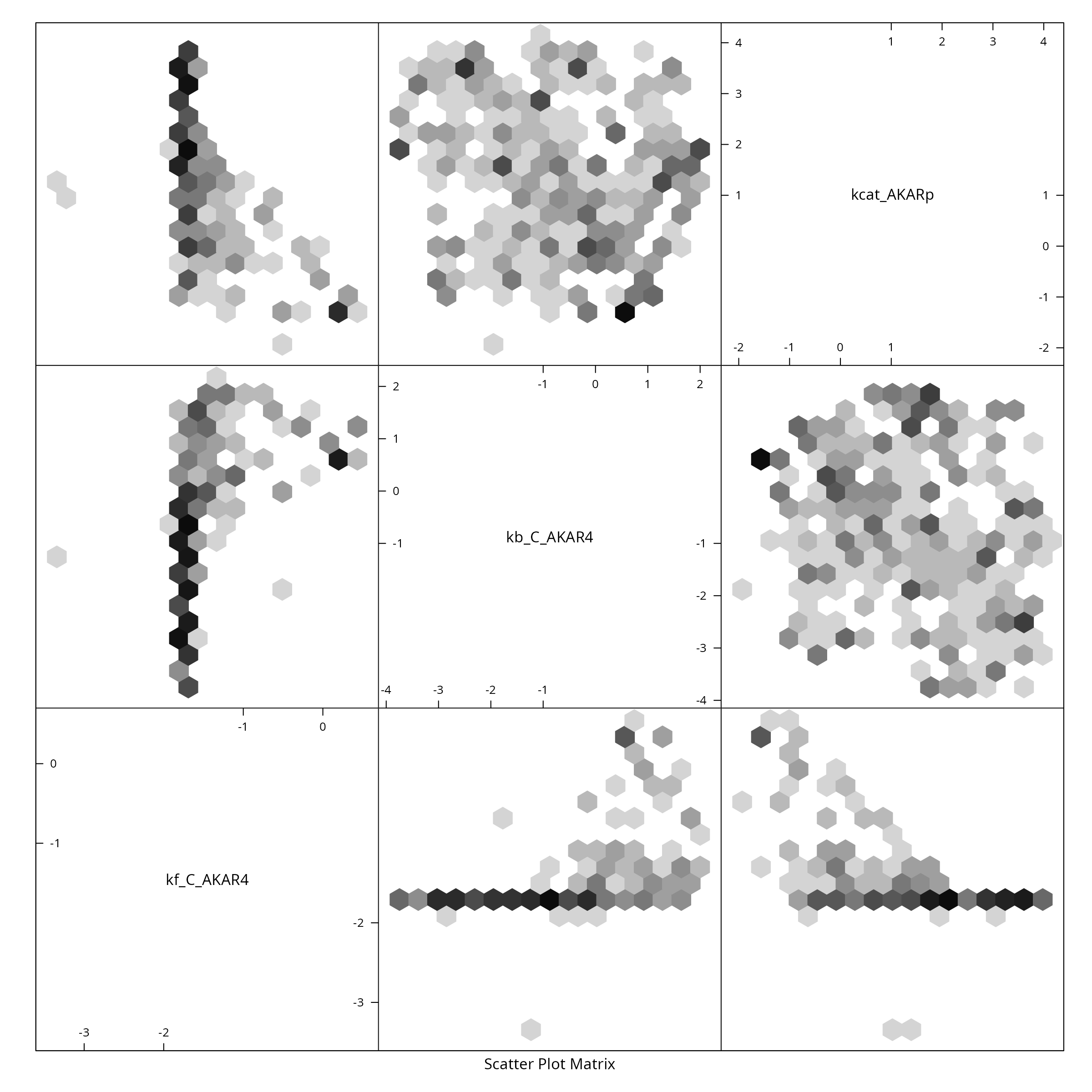
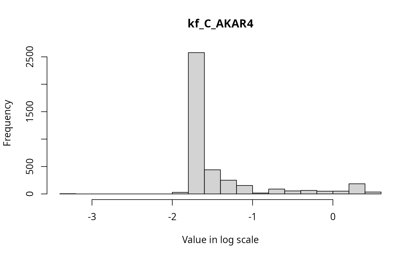
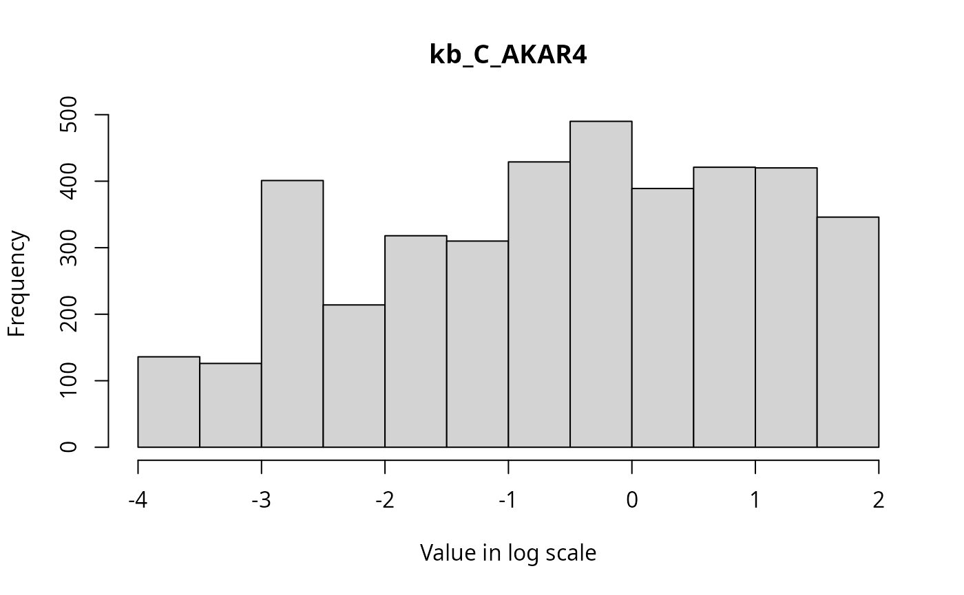
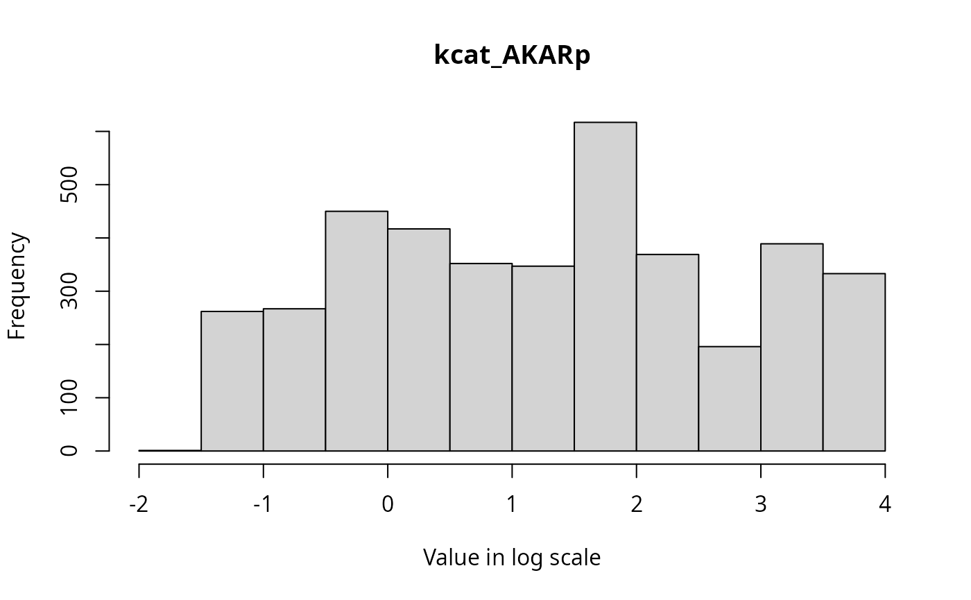
The marginal distributions of each parameter in the parameter vector can be visualized via histograms as follows.

for(i in 1:3){
 hist(ABCMCMCoutput$draws[,i], main=par_names[i], xlab = "Value in log scale")
}

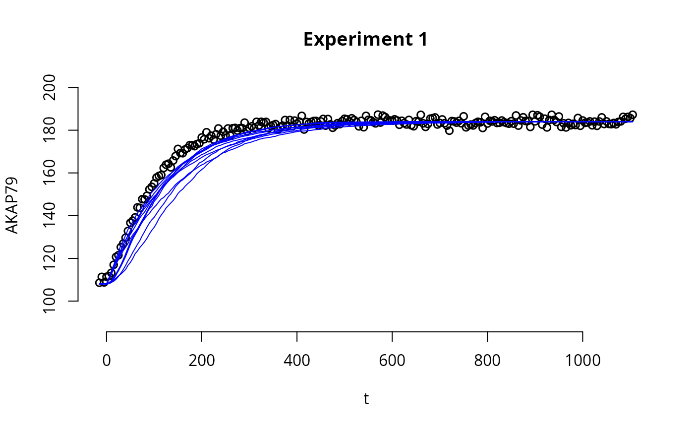
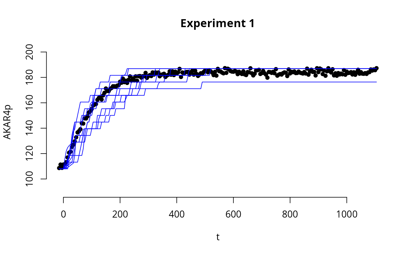
Simulate the stochastic model given posterior samples

To check the fit of the sampled posterior parameters with the experimental data, we can simulate trajectories given sampled parameters and compare them with the experimental data.


expInd <- 1 # Index of the experiment that we want to plot, with corresponding fitted trajectories
e <- experiments[[1]]

# Plot the experimental data
par(bty='n',xaxp=c(80,120,4))
plot(e$outputTimes, e$outputValues$AKAR4pOUT,ylim=c(90,200), ylab="AKAP79",
     xlab="t",
     main=sprintf("Experiment %i",expInd),
     lwd=1.5)

# generate a function (s) that simulates a trajectory given a parameter in input
s <- simulator.stoch(experiments = experiments, model.tab = SBtab, parMap = parMap, outputFunction = model$func, vol = vol, unit = unit, nStochSim = 3)

n_draws <- dim(ABCMCMCoutput$draws)[1] # number of sampled posterior parameters
subsample_indices <- sample(n_draws,10) # indices of 10 random parameters out of the paramneters in
for(i in subsample_indices){
  p <- ABCMCMCoutput$draws[i,] # random parameter from the posterior

  y <- s(p) # simulate a trajectory (y) given parameter p
  # "experiments" is a list of experiments
  # "y" is a list where element i of the list is a simulation performed with the experimental conditions as in the i-th element of list "experiments"
  
  lines(e$outputTimes, y[[expInd]]$output, col="blue") # plot the simulated trajectory
}