UQ for AKAR4 (stochastic model) • uqsa

library(uqsa)
library(errors)
library(parallel)

We use a particle filter (aka SMC) on the stochastic AKAR4 model, combined with ABC (due to the stochasticity of the model)

For information about the stochastic model, please read the article Simulate AKAR4 stochastically.

Load the Model

This model is included with the package, as one of the example models.

f <- uqsa_example("AKAR4")
m <- model_from_tsv(f)
ex <- experiments(m)

Make a Stochastic Version of AKAR4

sm <- as_cme(m)
C <- generate_code(sm)
c_path(sm) <- write_c_code(C)
#> Writing file: /tmp/RtmpiSVZvI/c7313866874d2944/AKAR4.c
so_path(sm) <- shlib(sm)
#> [1] "PKG_LIBS='-lgsl -lgslcblas -lm '"

To simulate the stochastic reaction network model we use the Gillespie algorithm.

Define MCMC settings

# scale to determine prior values
defRange <- 1000
par_val <- values(m$Parameter)

# Define Lower and Upper Limits for logUniform prior distribution for the parameters
ll <- c(par_val/defRange)
ul <- c(par_val*defRange)
ll = log10(ll) # log10-scale
ul = log10(ul) # log10-scale

# Define the prior distribution. In this case Uniform(ll,ul)
dprior <- dUniformPrior(ll, ul) # dprior evaluates the prior density function
rprior <- rUniformPrior(ll, ul) # rprior generates random samples from the prior

Generate an objective function

The objective function simulates the model, to do this it needs a simulator, it also needs direct access to the data, so ex is also an explicit arument for makeObjective:

s <- simstoch(
    ex, # list of experiments
    sm, # stochastic model, *with* shared library entry
    parMap=log10ParMap
)
objFunc <- makeObjective(ex,s)

Test evaluation of the objective function:

d <- objFunc(log10(values(m$Parameter)))
#> Warning: In 'Ops' : non-'errors' operand automatically coerced to an 'errors'
#> object with no uncertainty
print(d)
#>            [,1]
#> 400nM 0.2159661
#> 100nM 0.2150357
#> 25nM  0.1398377

It returns a vector of distance values (one per simulation experiment). But, when supplied with several parameters, it returns several columns:

D <- objFunc(t(rprior(7)))
print(D)
#>            [,1]      [,2]     [,3]      [,4]     [,5]      [,6]     [,7]
#> 400nM 0.2661257 0.4118178 0.484615 1.4853266 3.568595 0.4878092 0.475200
#> 100nM 0.2631928 1.6522022 1.949311 1.8469771 2.564294 1.9685288 1.904049
#> 25nM  0.2453741 3.0327972 4.455141 0.9200455 1.156957 4.5372318 4.287296

Run ABCSMC

We launch the particle filter from the prior (cold start), and pick resonable values for delta (the ABC distance threshold).

The data has measurement errors (standard error). The distance function takes the standard error into account, so the distances returned are relative, and expected to be close to 1. The function ABCSMC accepts two values for delta, an initial guess that is very permissive and a final value that triggers the SMC algorithm to terminate.

t_initial <- Sys.time()
options(mc.cores = detectCores())
X <- rprior(10000)
posterior <- ABCSMC(
    objFunc,
    startPar=t(X),
    Sigma=cov(X),
    delta=c(initial=3,final=0.5),
    dprior=dprior
)
t_final <- Sys.time()

cat(difftime(t_final,t_initial,units="min")," minutes")
#> 33.15168  minutes

Visualize the sampled parameters

The parameter-values in ABCMCMCoutput$draws are approximate samples from the posterior distribution, given the experiments.

The sampled three dimensional parameters for the AKAR4 model can be visualized via pairs of scatter plots, or two dimensional binning:

if (requireNamespace("hexbin")){
    hexbin::hexplom(posterior$draws, xbins = 24)
} else {
    pairs(posterior$draws, pch=20)
}
#> Loading required namespace: hexbin

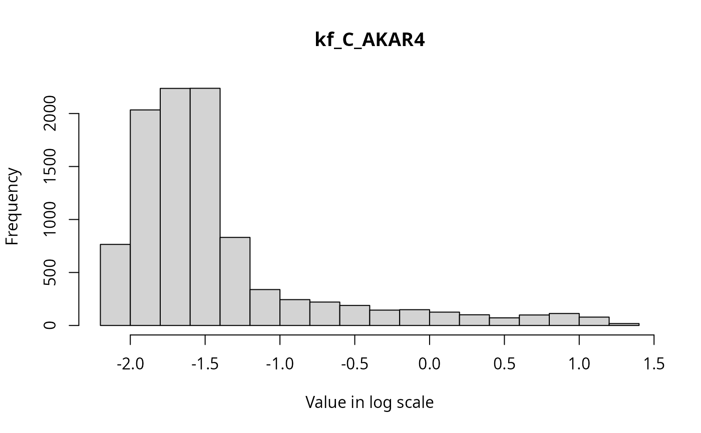
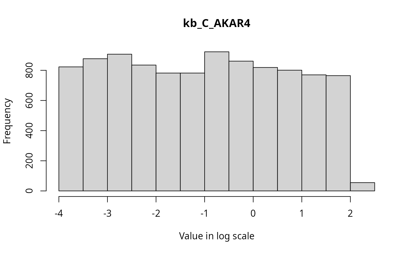
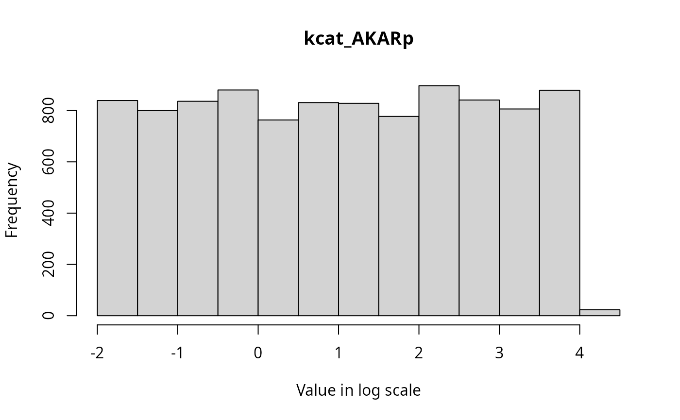
Marhinals

The marginal distributions of each parameter in the parameter vector can be visualized via histograms as follows.

for(i in seq_along(par_val)){
    hist(
        posterior$draws[,i],
        breaks = 20,
        main=names(par_val)[i],
        xlab = "Value in log scale"
    )
}

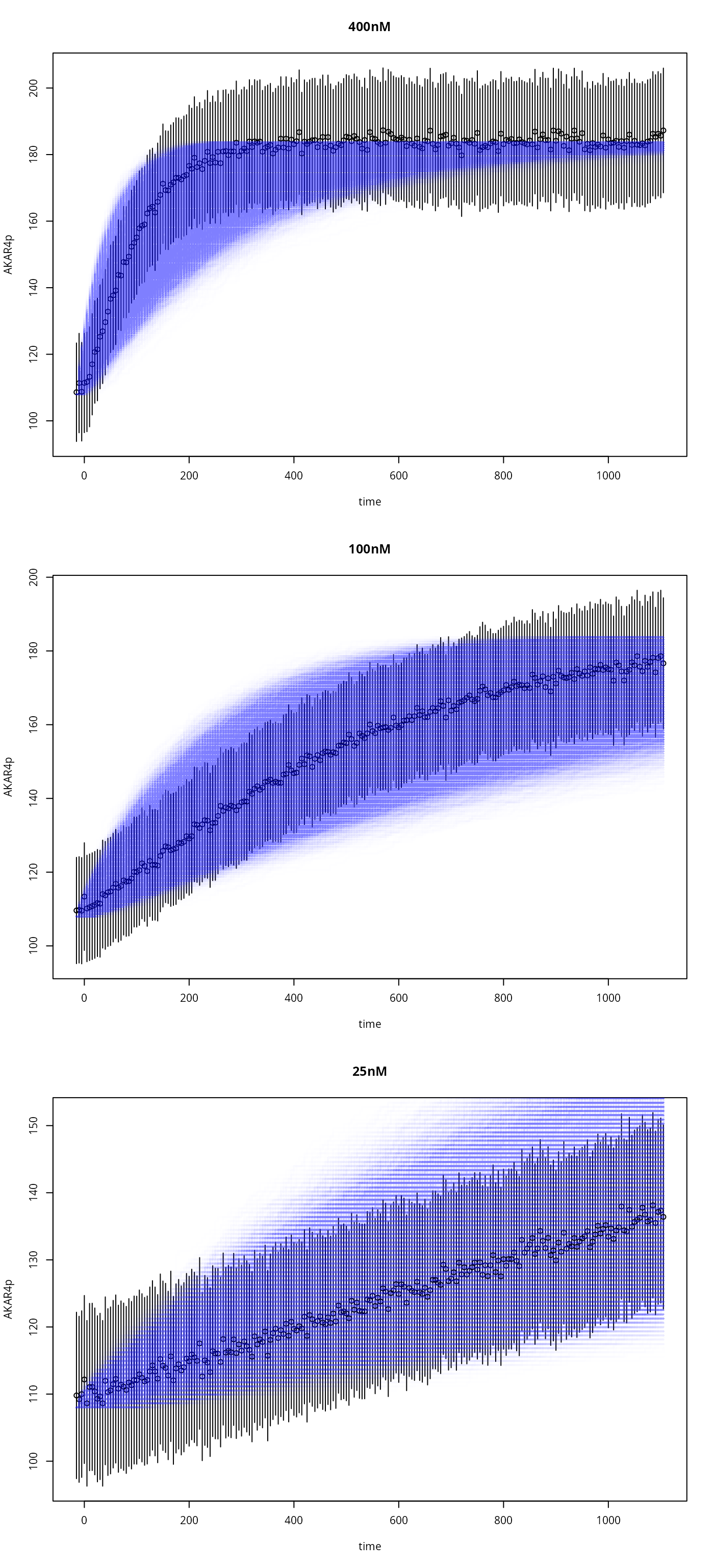
State Trajectories

t_initial <- Sys.time()
Z <- posterior$draws
y <- s(t(Z)) # using the stochastic simulator one final time
t_final <- Sys.time()

cat(difftime(t_final,t_initial,units="min")," minutes")
#> 0.1616517  minutes

par(mfrow=c(3,1))
for (i in seq_along(ex)){
    tm <- ex[[i]]$outputTimes
    plot(     # the data (errorbars)
        as.errors(tm),
        ex[[i]]$data,
        xlab="time",
        ylab="AKAR4p",
        main=names(ex)[i]
    )
    matplot(  # the simulation
        tm,
        drop(y[[i]]$func),
        type='s',
        col=rgb(50,50,200,1,max=255),
        lty=1,
        lwd=2,
        add=TRUE
    )
}