SMMALA and CaMKII

library(uqsa)

Simplified Manifold Metropolis Adjusted Langevin Algorithm

The included example model called CaMKII illustartes an insteresting case: - simulations are very different in consumed cpu time (by an order of magnitude) - simulation time heavily depends on the used solver - the data type is Dose Response rather than Time Series - simulations are very slow compared to the other example models

This makes the likelihood function (or objective function) expensive. For this reason, we need to make high quality Markov chain proposals, to increase the impact that a single likelihood evaluation makes.

The SMMALA algorithm tries to address this issue and provide update proposals that traverse a larger distance than what is feasible with the metropolis algorithm while keeping the same acceptance rate.

These higher quality proposals are informed by the gradient of the log-likelihood, and its Fisher information matrix.

An ingredient of the Fisher information is the solution’s sensitivity

\[S(t;x,p)_i^{~j} = \frac{d x_i(t;p)}{dp_j}\,,\]

which is usually quite difficult to get. Instead we approximate it. The rgsl package will try to approximate the sensitivity in a deterministic way. The approximation error will make the overall algorithm less efficient than using exact solutions, but the approximations are better the closer we are to a steady state.

In this model the data is either in steady state, or very close to it, so the approximations work very well.

The default parameters are not optimized to fit the data. We don’t expect a good fit in the initial simulation.

Below we describe two different approaches for this model. Ultimately, the frist approach makes better use of compute-resources.

The model is very sensitive to integrator choices, some perform better some worse. It is very likely that the sundials solvers would perform much better than the GSL solvers, but even between different GSL solvers there are big differences in consumed cpu-time.

Dose Sequence Approach

For this model one of th epossible approaches is to create an event schedule that applies a certain dose of base calcium or calmodulin (depending on the experiment) in a sequence. Here is an example dose sequence of base Ca levels (dose column):

id       time  transformation       dose
ShTP01      0      CaSeq            364
ShTP02      10     CaSeq            2305
ShTP03      20     CaSeq            2548
ShTP04      30     CaSeq            2912
ShTP05      40     CaSeq            3640
ShTP06      50     CaSeq            4126
ShTP08      70     CaSeq            4611
ShTP10      90     CaSeq            5461
ShTP12      110    CaSeq            6067
ShTP14      130    CaSeq            6796
ShTP16      150    CaSeq            7281
ShTP17      160    CaSeq            8495
ShTP18      170    CaSeq            9344
ShTP19      180    CaSeq            24393
ShTP20      190    CaSeq            34101

The transformation event CaSeq is defined in the third row of Transformation.tsv (named CaSeq):

id      CaBase   CaM_0
CaSeq   dose     CaM_0
CaMSeq  CaBase   dose

where the column-header identifies the quantity to set, and the expressions below provide the value. The special variable dose is a scalar that can be set for each event in the schedule (previous table).

We represent each experiment as a time series, even though the data sets were originally represented as dose response curves (a map between an input [e.g. Ca] and an output [e.g. ActivePP2B]). We arbitrarily set a time betwen input doses and simulate all points in one series, with just enough time in-between to reach the next higher steady state from the current steady state (the steady state level changes with each dose of base-level Ca).

The table of experiments looks like this (truncated):

id                  type         PP1_0   CaMKII_0   CaM_0   PP2B_0   isOn    t0  event
Bradshaw2003Fig2E   Time Series  0       200        2000    0        TRUE   -60  EventScheduleBradshaw2003Fig2E
Shifman2006Fig1Bsq  Time Series  0       5000       5000    0        TRUE   -60  EventScheduleShifman2006Fig1Bsq
ODonnel2010Fig3Co   Time Series  0       0          0       100      FALSE  -60  EventScheduleODonnel2010Fig3Co
Stemmer1993Fig1tr   Time Series  0       0          300     3        TRUE   -60  EventScheduleStemmer1993Fig1tr
Stemmer1993Fig1fc   Time Series  0       0          30      3        TRUE   -60  EventScheduleStemmer1993Fig1fc
Stemmer1993Fig2Afc  Time Series  0       0          25000   0        TRUE   -60  EventScheduleStemmer1993Fig2Afc

Simulation

During a simulation, these doses will create a staircase of (local) equilibria:

library(parallel)

f  <- uqsa_example("CaMKIIs")
m <- model_from_tsv(f)
o <- as_ode(m)
#> Loading required namespace: pracma
ex <- experiments(m,o)
C <- generate_code(o)
c_path(o) <- write_c_code(C)
so_path(o) <- shlib(o)

print(length(ex))
#> [1] 6
options(mc.cores = length(ex))

p <- values(m$Parameter) # in log-space
stopifnot(all(m$Parameter$scale=="ln"))

A Time-Dense Simulation

This is a simulation with time points inserted between the measurement times, to see what happens in-between them:

for (i in seq_along(ex)){
    t_ <- ex[[i]]$outputTimes
    ex[[i]]$measurementTimes <- t_ # save old values for later
    ex[[i]]$outputTimes <- sort(
        c(
            t_,
            seq(0,max(t_),length.out=length(t_)*10)
        )  # 10x time-points
    )
}

s <- simulator.c(ex, o, parMap=logParMap)
y <- s(p)

cpuSeconds <- unlist(lapply(y,\(l) l$cpuSeconds))
names(cpuSeconds) <- names(ex)

print(cpuSeconds)
#>  Bradshaw2003Fig2E Shifman2006Fig1Bsq  ODonnel2010Fig3Co  Stemmer1993Fig1tr 
#>           0.019591           0.013567           0.014327           0.006781 
#>  Stemmer1993Fig1fc Stemmer1993Fig2Afc 
#>           0.008960           0.035513

Next, we plot the results of that dense simulation:

par(mfrow=c(3,2), bty="n")
for (i in seq_along(ex)){
    j  <- rownames(m$Output) %in% colnames(ex[[i]]$measurements)
    t_siml <-ex[[i]]$outputTimes
    f_siml <-y[[i]]$func[j,,1]
    t_data <-ex[[i]]$measurementTimes
    plot(
        errors::as.errors(t_data),
        ex[[i]]$data[j,],
        main=names(ex)[i],
        xlab="t",
        ylab=rownames(m$Output)[j]
    )
    lines(t_siml,f_siml,col='red4')
}

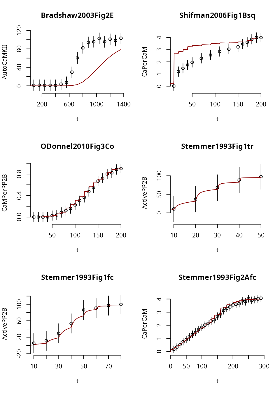
Here we notice that in Experiment 1, the trajectory fails to reach steady state (i.e. a flat line), for any dose. So, it doesn’t look like a staircase at all. This may or may not be desireable (depends on whether the original experiment was in steady state).

Because most data-structures are just plain R data types, it is easy to modify experiments and experiment with the simulations. Here we make the entire time-course longer

ex[[1]]$events$time <- ex[[1]]$events$time*60
ex[[1]]$outputTimes <- ex[[1]]$outputTimes*60
ex[[1]]$measurementTimes <- ex[[1]]$measurementTimes*60

Becasue we changed the experimental setup, we recreate the solver function:

s <- simulator.c(ex, o, parMap=logParMap)
y <- s(p) # new solution

We repeat the same plot from above:

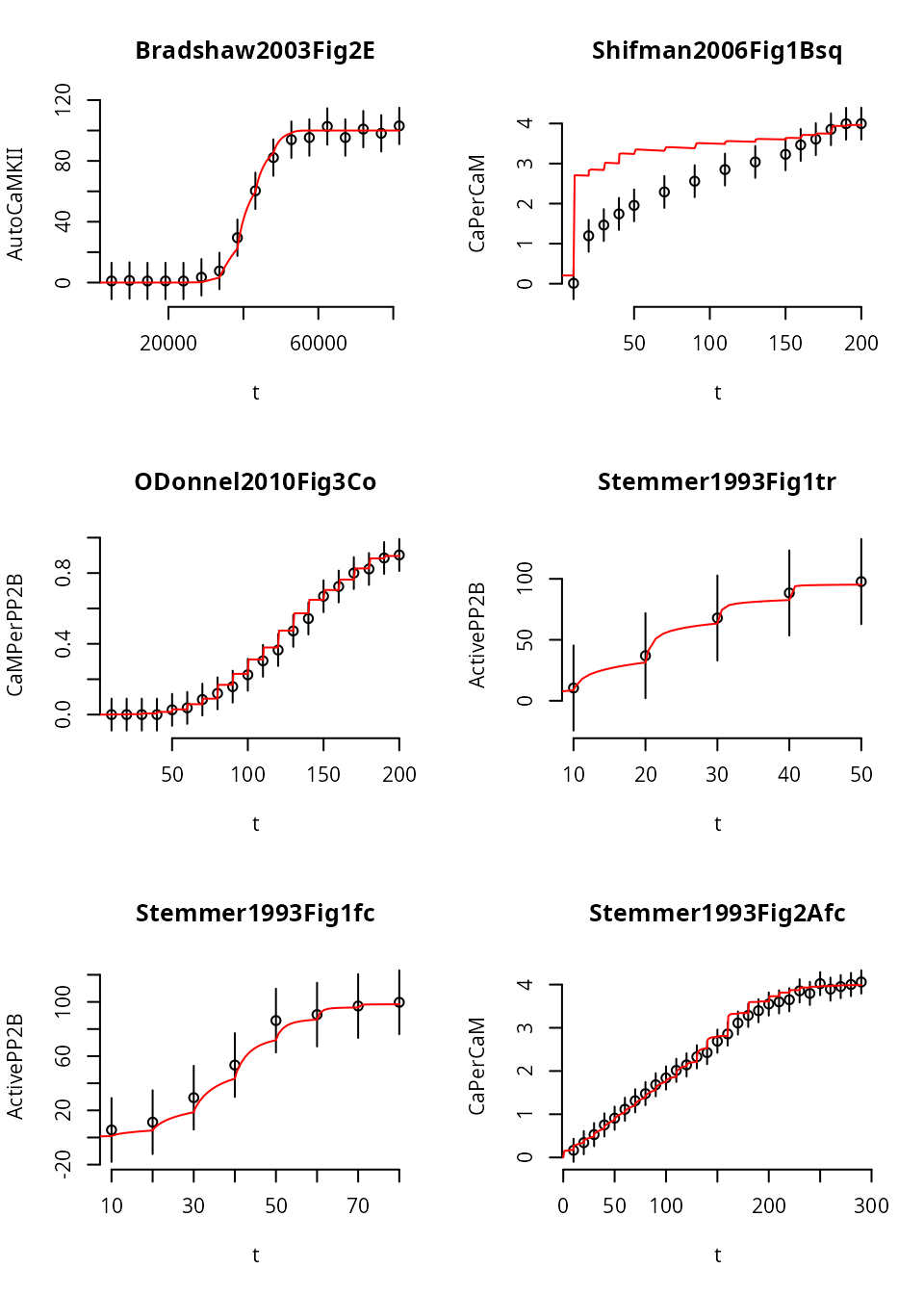
Giving this experiment more time shifts the simulated model response, but doesn’t produce a steady state (yet).

It is possible that the default parameter set will not allow the system to go into steady state quickliy enough, even if we increase the time between the transformation events more. On the other hand, the original data was measured with \(600\,\text{s}\) equilibration time, not in verified steady state.

Asymmetry

The experiments for this model are different in complexity. How many seconds the solver needs to claculate a simulated trajectory depends on the chosen integration method.

Solver timings for CaMKIIs, with indicated Success and Failure.

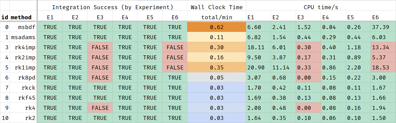
This Table-screenshot shows that some of the integration methods fail to return a solution for some of the simulated scenarios, even with the default parameters. These methods should be excluded from MCMC. The remaining methods perform very differently. Some of these methods may fail for parameter-vectors proposed during MCMC.

This al means that the posterior distribution depends on the used solver: no solution from the chosen solver means that the liklelihood is 0. So, it may be a good idea to use the most robust solver if it means that more solutions are found.

This is a table of acceptable cpu times in seconds:

CPU time measured in seconds, tabulated by experiment for different step methods. Only Successful simulations are shown. {#tbl:cpu-time}

id	method	Exp 1	Exp 2	Exp 3	Exp 4	Exp 5	Exp 6
0	msbdf	6.603	2.41	1.522	0.035	0.265	37.386
1	msadams	6.822	1.54	0.435	0.287	0.437	6.033
7	rkck	1.703	0.419	0.113	0.077	0.109	1.669
8	rkf45	1.692	0.385	0.129	0.08	0.125	1.656
10	rk2	1.642	0.347	0.104	0.063	0.102	1.498

This table shows that it is vitally important to pick the right integration method, but also that simulating experiments in parallel is not always a good idea as some of the threads will return much sooner than others and idle until the slowest experiment is finished. Starting more Markov chains may be better in that case.

Here is an example, where we stretched the time-line for the Experiment named Bradshaw2003Fig2E as it is very slow to approach steady state and the most problematic experiment in this dose sequence.

Stretching the time line allows the ODE system more time to converge, but also increases the simulation time:

Stretched time line for Experiment 1 (event-shedule and measurement times).

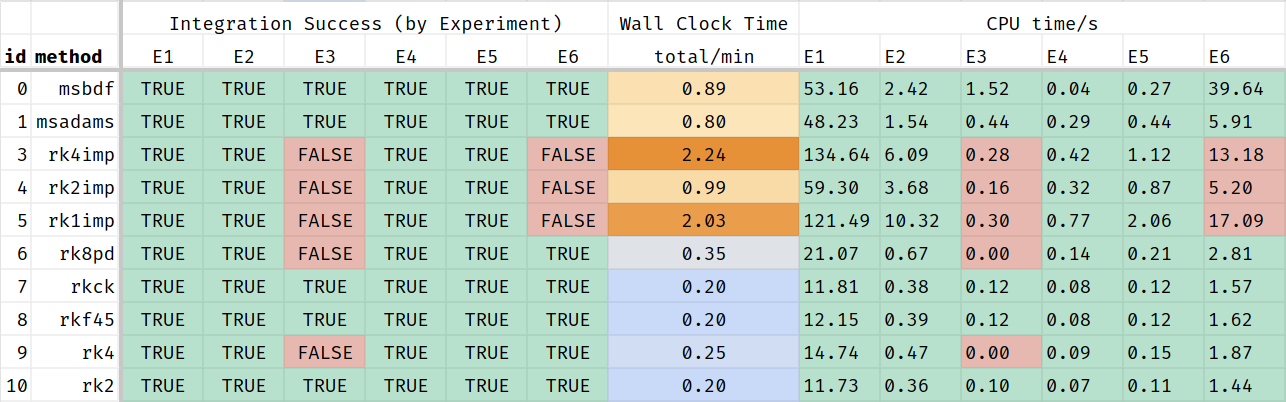
And again, just the portion where all experiments returned a result:

CPU time measured in seconds, tabulated by experiment for different step methods. Only Successful simulations are shown. {#tbl:cpu-time-stretched-1}

id	method	Exp 1	Exp 2	Exp 3	Exp 4	Exp 5	Exp 6
0	msbdf	53.16	2.42	1.52	0.04	0.27	39.64
1	msadams	48.23	1.54	0.44	0.29	0.44	5.91
7	rkck	11.81	0.38	0.12	0.08	0.12	1.57
8	rkf45	12.15	0.39	0.12	0.08	0.12	1.62
10	rk2	11.73	0.36	0.10	0.07	0.11	1.44

Dose Response Approach

Instead, we can also simulate this model as a dose response curve. This is done in a copy of the model that doens’t have the s suffix (for sequential).

In this formulation of the model, we need to be able to reach each steady state from the default initial conditions, not just from a very nearby previous steady state. So, we give the system more time to reach it (600 seconds !Time for each data point). Because of this longer time, this is a less efficient approach. The advantage is that it avoids event schedules and transformations entirely.

id                  type           Ca_set   PP1_0   CaMKII_0   CaM_0   PP2B_0   cab    t0   event   time
Bradshaw2003Fig2E   Dose Response  -1       0       200        2000    0        0     -100  TurnOn  600
Shifman2006Fig1Bsq  Dose Response  -1       0       5000       5000    0        0     -100  TurnOn  600
ODonnel2010Fig3Co   Dose Response  0        0       0          -1      100      0     -100  TurnOn  600
Stemmer1993Fig1tr   Dose Response  -1       0       0          300     3        0     -100  TurnOn  600
Stemmer1993Fig1fc   Dose Response  -1       0       0          30      3        0     -100  TurnOn  600
Stemmer1993Fig2Afc  Dose Response  -1       0       0          25000   0        0     -100  TurnOn  600

The data files look different, they map inputs to outputs, rather than time to outputs:

id     Ca_set   AutoCaMKII
E0D0   175.8    1.04;11.9953
E0D1   236      1.38;11.9953
E0D2   313.3    1.04;11.9953
E0D3   426.6    1.04;11.9953
E0D4   564.9    1.04;11.9953
E0D5   749.9    3.46;11.9953
E0D6   1006.9   7.63;11.9953
E0D7   1336.6   29.47;11.9953
E0D8   1794.7   60.34;11.9953
E0D9   2349.6   82.19;11.9953
E0D10  3198.9   93.98;11.9953
E0D11  4246.2   95.37;11.9953
E0D12  5623.4   102.65;11.9953
E0D13  7568.3   95.37;11.9953
E0D14  10303.9  100.92;11.9953
E0D15  13489.6  98.15;11.9953
E0D16  18113.4  103;11.9953

In this version of the model, there are no events at all. This sequence of Ca doses will be converted to one time series experiment per line; the dose id will be used as part of the experiment name.

Each point is treated as an independent measurement, unrelated to its neighbors. The doses and data points can be in any order.

f  <- uqsa_example("CaMKII") # no 's'
m <- model_from_tsv(f)
o <- as_ode(m)
ex <- experiments(m,o)
#>                             type  event
#> Bradshaw2003Fig2E  dose response TurnOn
#> Shifman2006Fig1Bsq dose response TurnOn
#> ODonnel2010Fig3Co  dose response TurnOn
#> Stemmer1993Fig1tr  dose response TurnOn
#> Stemmer1993Fig1fc  dose response TurnOn
#> Stemmer1993Fig2Afc dose response TurnOn
#> Warning in dose_response_experiments(m, E[l, , drop = FALSE], iv[, l, drop =
#> FALSE], : Dose response experiments are not (yet) fully compatible with events,
#> this script will try its best.
print(length(ex))
#> [1] 100

options(mc.cores = detectCores())
c_path(o) <- write_c_code(generate_code(o))
so_path(o) <- shlib(o)
p <- values(m$Parameter)

Simulate a subset of experiments (those that start with E0):

i <- which(startsWith(names(ex),"Bradshaw"))
s <- simulator.c(ex[i],o,parMap=logParMap)
y <- s(p)

cpuSeconds <- Reduce(\(a,b) a+b$cpuSeconds,y,init=0.0)
print(cpuSeconds)
#> [1] 0.033741

The simulation time is very slightly longer than before, because each final point needs to equilibrate individually. We plot the dose response, by collecting it from the solution:

j <- rownames(m$Output) %in% colnames(ex[[i[1]]]$measurements)
Ca <- unlist(lapply(ex[i],\(x) x$input['Ca_set']))
f_ <- unlist(lapply(y,\(y) y$func[j,1,1]))
v_ <- unlist(lapply(ex[i],\(x) x$data[j,1]))

par(bty="n")
plot(
    Ca,
    v_,
    main=names(ex)[i[1]],
    xlab="Ca",
    ylab=paste(rownames(m$Output)[j],collapse=" "),
    log="x"
)
points(Ca,f_,pch=2,col="red4")

Here the triangles represent the independent simulation results.

This approach lends itself more to parallelization than the dose sequence, because all these independent points can be simulated in parallel (all 99 points, within each curve and between the curves). But, if a small number of the points require a long simulation time, then their solution will pause the entire Markov chain until all points have been obtained.

Therefore, it may be much better to simulate all experiments sequentially (see previous section), and instead start more parallel Markov chains (and merge them in the end). This way, fewer MPI-workers/threads/cores idle.