Uncertainty Quantification and global Sensitivity Analysis on AKAR4 (deterministic)
uqsaAKAR4.RmdLoad Model and Data
First we load the model and data, for detailed explanations see previous examples (Simulate AKAR4 deterministically).
f  <- uqsa_example("AKAR4")
m <- model_from_tsv(f)
o <- write_and_compile(as_ode(m))
#> Loading required namespace: pracma
ex <- experiments(m,o)Uncertainty quantification: Sample the posterior distribution
For details on how to sample from the posterior distribution, see, e.g., the deterministic AKAR4 example. First we construct the prior. For this article, we override the information in the file and pick an iid normal prior with \(\sigma=2\) for all parameters:
sd <- rep(2,length(p))        # sigma = 2
dprior <- dNormalPrior(p,sd)
rprior <- rNormalPrior(p,sd)
mh <- mcmc(                   # metropolis hastings
    metropolis_update(        # random walk
        s,
        dprior=dprior,
        Sigma=diag(sd^2)
    )
)
We obtain a high quality sample by following the steps described in details in the deterministic AKAR4 example). This will take a minute or so on a laptop.
set.seed(137)
x <- mcmc_init(beta=1.0,p,s,ll,dprior)
h <- tune_step_size(mh,x)
#> acceptance rate: 0.99, step-size: 0.0001;
#> acceptance rate: 1, step-size: 0.000188011;
#> acceptance rate: 1, step-size: 0.000353903;
#> acceptance rate: 0.98, step-size: 0.00066617;
#> acceptance rate: 0.98, step-size: 0.00125093;
#> acceptance rate: 1, step-size: 0.002349;
N <- 3e4

nCores <- parallel::detectCores()

bigSample <- parallel::mclapply(
    seq(nCores),
    function(i) {
        return(mh(x,N,h))
    },
    mc.cores=nCores
)

S_ <- Reduce(\(a,b) {rbind(a,b)},bigSample,init=NULL)
L_ <- Reduce(\(a,b) {c(a,attr(b,"logLikelihood"))},bigSample,init=NULL)
colnames(S_) <- names(p)
We should estimate the auto-correlation of this sample, to reduce the size effectively, for plotting and post-processing:
if (require(hadron)){
    res <- uwerr(data=L_)
    tau <- ceiling(res$tauint + res$dtauint)
} else {
    A <- acf(L_,lag.max=1000)
    i <- which(A$acf < exp(-3))[1]
    tau <- ceiling(sum(A$acf[seq(i)]))
}
#> Loading required package: hadron
#>
#> Attaching package: 'hadron'
#> The following object is masked from 'package:base':
#>
#>     kappa

print(tau)
#> [1] 69

if (1 < tau && tau < length(L_)){
    N <- length(L_)
    S_ <- S_[seq(1,N,by=tau),]
    L_ <- L_[seq(1,N,by=tau)]
    N <- length(L_)
}
Pairs plot (either with hexagonal binning or normal)
if (require(hexbin)){
    hexbin::hexplom(S_)    # binning
} else {
    pairs(
        S_,                # the sample
        pch=16,            # filled circle
        ces=4,             # so that points overlap
        col=rgb(0,0,1,0.1) # transparent blue
    )
}
#> Loading required package: hexbin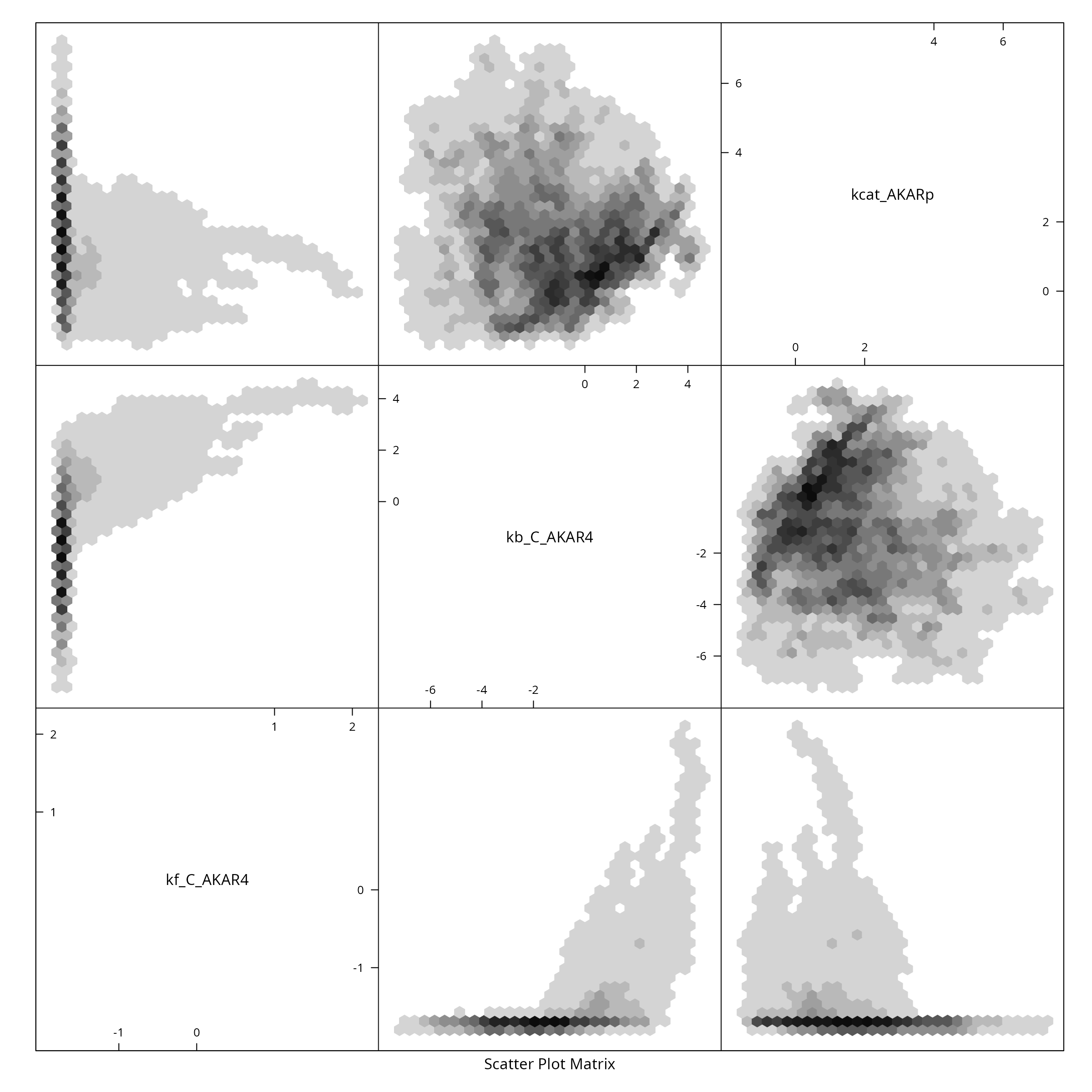
Sensitivity analysis on the posterior distribution
First we need to (re-)create the simulation result corresponding to the posterior parameter sample. This will take a minute or so on a laptop.
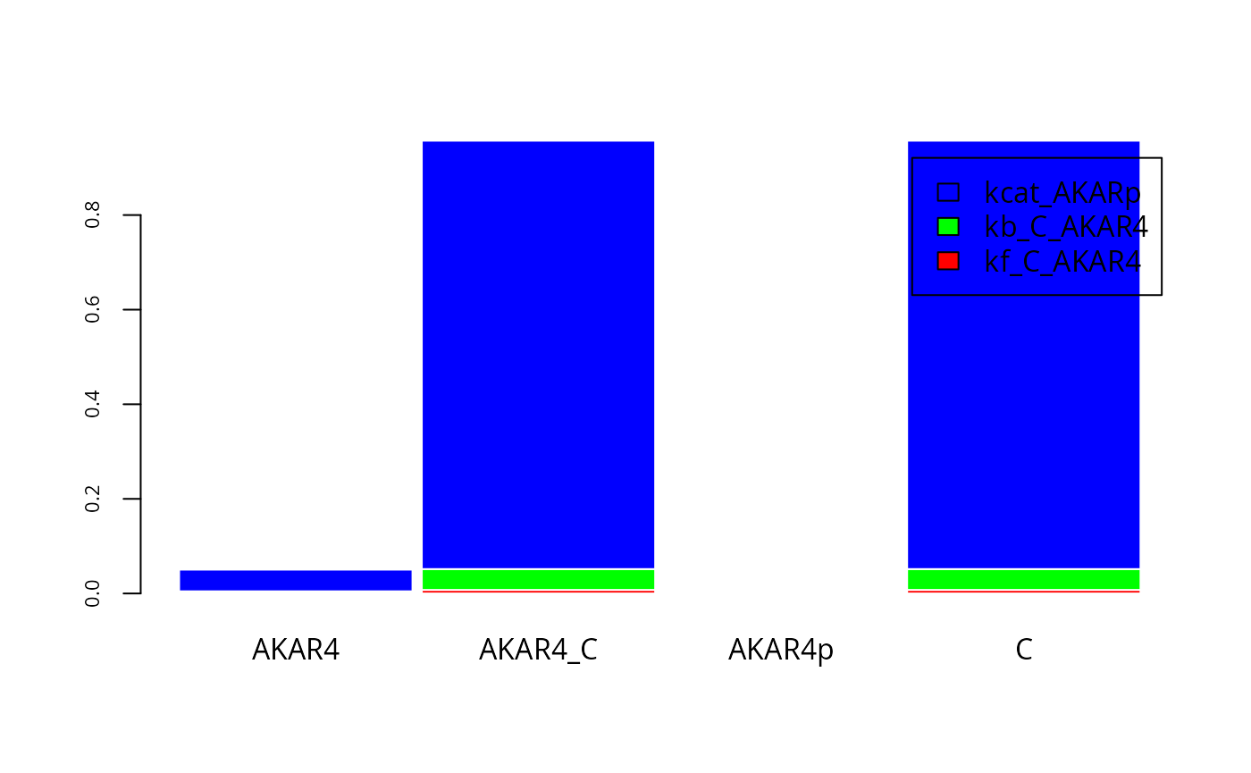
y <- s(t(S_))Next we calculate the first order sensitivity indexes. Here for compute them for a specific experimental setting and time point:
E <- 2                      # Experiment idx
T <- 60                     # Time idx
fM <- y[[E]]$state[,T,]
SIappr <- gsa_binning(S_, t(fM))
and plot the result:
cols=rainbow(3)
par(mfrow = c(1, 1))
fM <- y[[E]]$state[,T,]
barplot(
    t(SIappr),
    col=cols,
    border="white",
    space=0.04,
    cex.axis=0.7,
    legend.text=names(p)
)
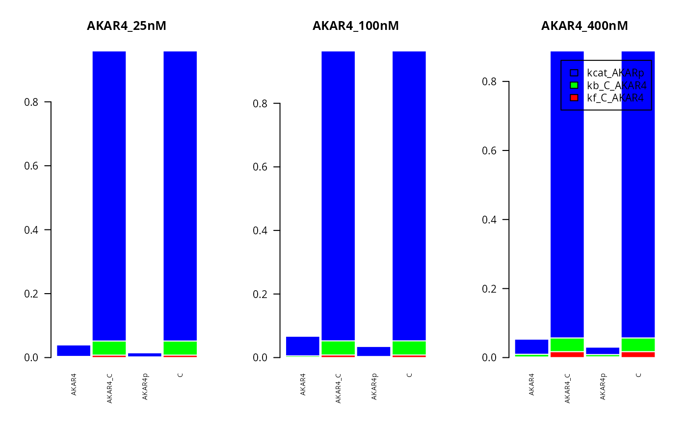
Here for compute the first order sensitivity indexes for all three experiments, looking at the different compounds in the system (on the x axis):
T <- 200                    #Time idx
par(mfrow = c(1,3))
for (E in seq(3,1,-1)){
fM <- y[[E]]$state[,T,]
SIappr <- gsa_binning(S_, t(fM))
lgd <- list(names(p), NULL,NULL)
barplot(
    t(SIappr),
    col = cols,
    cex.names = 0.7,
    las = 2,
    border = "white",
    space = 0.04,
    cex.axis = 1,
    main = names(ex)[E],
    legend.text = lgd[[E]])
}
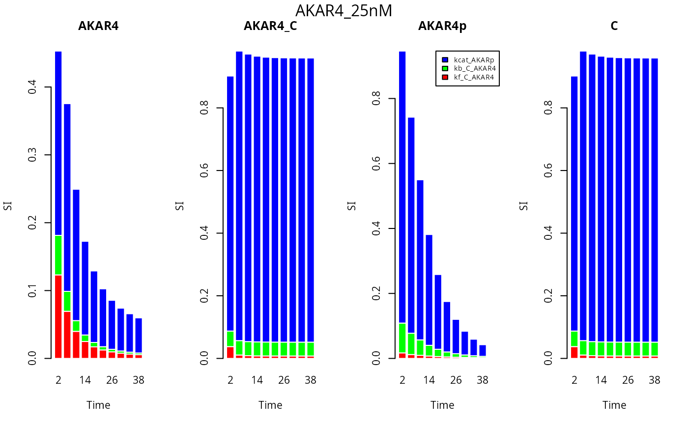
Now we investigate the first order sensitivity indexes at different time points (time is on the x axis) for each of the compounds and one experiment.
E <- 3
timePts <- seq(2,40,by=4)  #Avoid first time point
nStates=dim(y[[E]]$state)[1]
cols=rainbow(3)
par(mfrow = c(1, nStates))
lgd <- rep(list(NULL),nStates)
lgd[[nStates-1]] <- names(p)
for (Cm in seq(nStates)) {
    fM <- y[[E]]$state[Cm,timePts,]
    SIappr <-gsa_binning(S_, t(fM))
    names(SIappr) <- timePts
    barplot(
        t(SIappr),
        col=cols,
        names.arg = timePts,
        border="white",
        cex.axis=1,
        main=dimnames(y[[E]]$state)[[1]][Cm],
        xlab="Time",
        ylab="SI",
        legend.text=lgd[[Cm]],
        args.legend = list(x = "topright", inset=c(-0.1, 0), cex=0.7)
    )
}
mtext(names(ex[E]), side=3, line = - 1.5, outer=TRUE)