Global sensitivity analysis on AKAR4 - independent input factors • uqsa

library(uqsa)
library(SBtabVFGEN)
library(rgsl)
library(ggplot2)

This article provides code do perform global sensitivity analysis with the Sobol-Saltelli method and the with the binning-approach.

Load the SBtab files, create ODE model code and load examples similar to the example Simulate the AKAR4 deterministic model.

modelFiles  <- uqsa::uqsa_example("AKAR4")
SBtab <- SBtabVFGEN::sbtab_from_tsv(modelFiles)
model  <- SBtabVFGEN::sbtab_to_vfgen(SBtab, cla=FALSE)
experiments <- SBtabVFGEN::sbtab.data(SBtab)
C <- uqsa::generateCode(model)
cat(C,sep="\n",file="./AKAR4_gvf.c")
modelName <- checkModel("AKAR4",modelFile="./AKAR4_gvf.c")

Create simulator

We construct a simulator function and and test it on default parameter values.

s <- simcf(experiments,modelName,parMap=log10ParMap) # or simulator.c
p <- log10(SBtab$Parameter[["!DefaultValue"]])
names(p) <- rownames(SBtab$Parameter)
y <- s(p) # here the simulation happens

Set meta-parameters for the global sensitivity simulation

nSamples <- 40000

nSamples corresponds to the number of samples in M1 (or M2) of the Soboll-Saltelli approach..The number of simulations of the Sobol-Saltelli approach consists of 2*nSampels+nPars*nSamples number of simulations. In the binning approach below we use 2*nSamples number of samples (corresponding to 2*nSamples number of simulations) to use the same number of independent sample points as Sobol-Saltelli.

Construct parameter prior samples according to Sobol-Saltelli (M1, M2, N).

nPars <- length(p)
rprior <- rNormalPrior(p, array(1, nPars))
prior <- saltelli_prior(nSamples, rprior)
names(prior)
#> [1] "M1" "M2" "N"

Plot parameter prior (M1)

title<-paste("Prior distribution experiment");
boxplot(prior$M1, main = title, names=names(p), las=2, cex.main=0.9, cex.axis=0.3)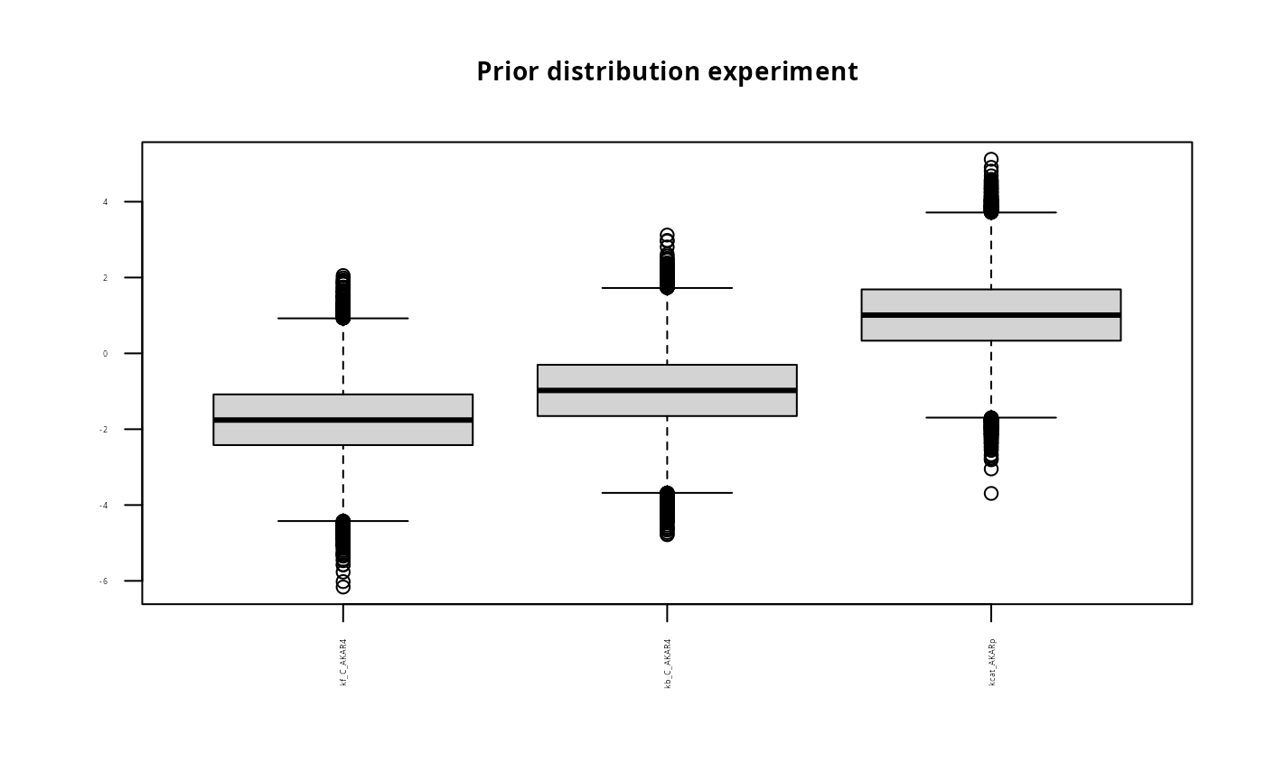

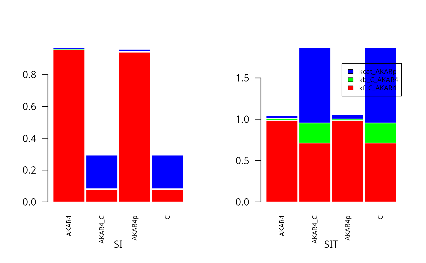
Simulate from the prior

Set up simulator considering one experiment

expIdx <- 2 #experiment to look at
s <- simcf(experiments[expIdx],modelName,parMap=log10ParMap)
#Test by simulting the default parameter set:
p <- log10(SBtab$Parameter[["!DefaultValue"]])
names(p) <- rownames(SBtab$Parameter)
y <- s(p) # here the simulation happens

Use states (compound concentrations) as output and look at one time point alone

T <-5 #timepoint to investigate
nStates <- dim(y[[1]]$state)[1]
fM1 <- t(s(t(prior$M1))[[1]]$state[,T,])
fM2 <- t(s(t(prior$M2))[[1]]$state[,T,])
fN <- array(NA, dim=c(nSamples,nStates, nPars))
for (i in 1:nPars){
  print(i)
  fN[,,i] <- t(s(t(prior$N[,,i]))[[1]]$state[,T,])
}
#> [1] 1
#> [1] 2
#> [1] 3

Calculate and plot sensitivity indexes

Calculate sensitivity indexes for sobol-saltelli

SA <- gsa_saltelli(fM1,fM2,fN)

Plot first (SI) and total-order (SIT) sensitivity indexes for sobol-saltelli

cols=rainbow(3)
par(mfrow = c(1, 2))
barplot(t(SA$SI[,]), 
        col=cols,
        border="white", 
        space=0.04, 
        cex.axis=1,
        names.arg=dimnames(y[[1]]$state)[[1]],
        cex.names = 0.7,
        las = 2,
        xlab="SI",  las=2, cex.main=0.9)
barplot(t(SA$SIT[,]), 
        col=cols, 
        border="white", 
        space=0.04, 
        cex.axis=1,
        names.arg=dimnames(y[[1]]$state)[[1]],
        cex.names = 0.7,
        las = 2,
        xlab="SIT",
        legend.text=SBtab$Parameter[,1],
        args.legend = list(x = "topright", inset=c(0, 0.1), cex=0.7))

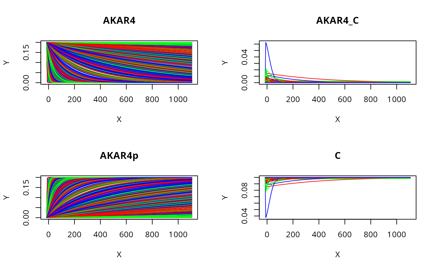
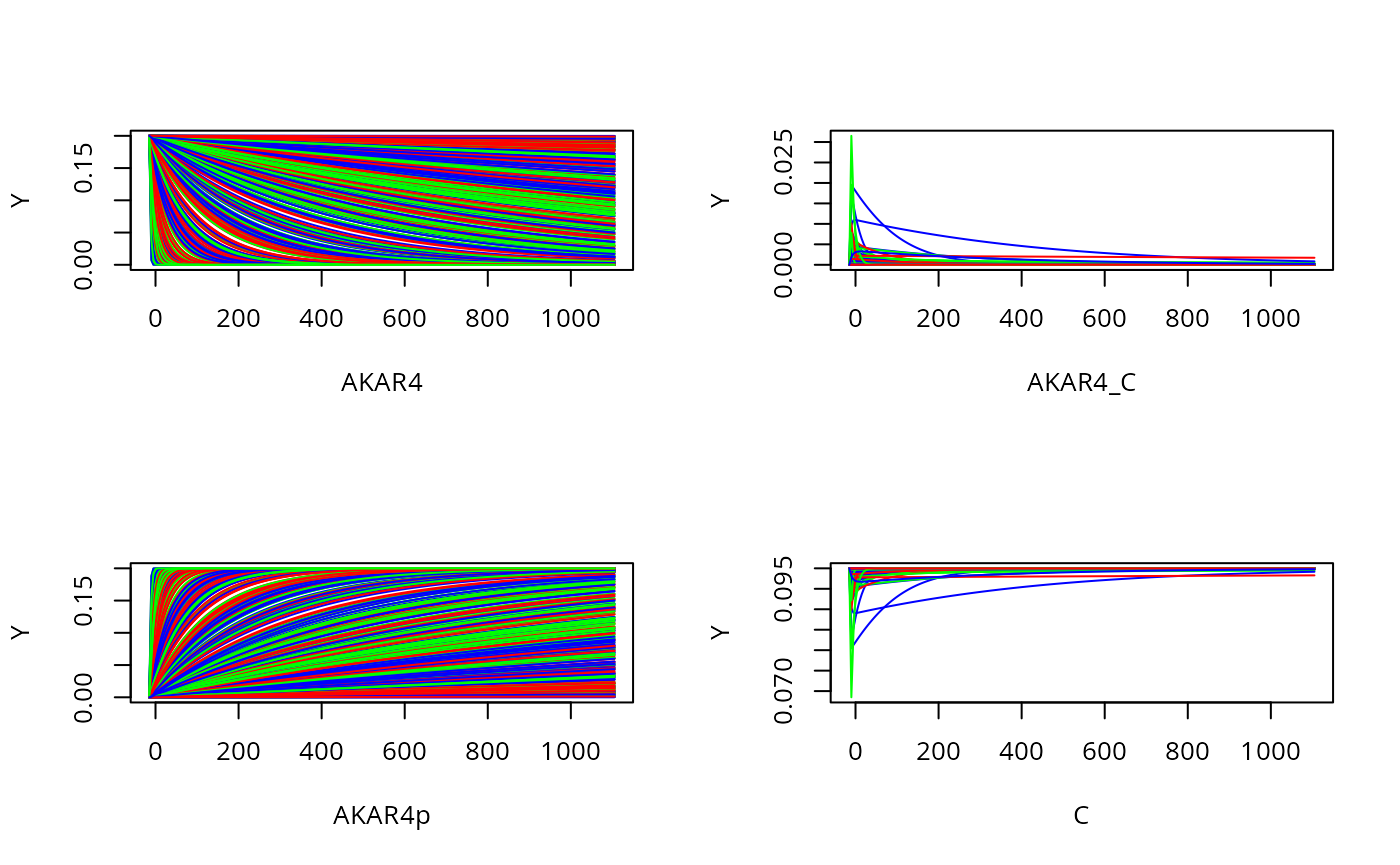
Plot all states and timeponts for the experiment

allTimesSample=s(t(prior$M2))[[1]]$state
par(mfrow = c(2, 2))
for (i in 1:4) {
matplot(experiments[[1]]$outputTime,allTimesSample[i,,1:500] , type = "l", lty = 1, 
        col = c("red", "blue", "green"), 
        ylab = "Y", xlab= dimnames(allTimesSample)[[1]][i])
}

Calculate first order sensitivity index (SI) based on binning approach

SIappr <-gsa_binning(rbind(prior$M1,prior$M2), rbind(fM1,fM2), nBins = "Sturges")

Plot SI for Sobol-Saltelli versus the binning approach

par(mfrow = c(1, 3))
barplot(t(SA$SI[,]), 
        col=cols, 
        border="white", 
        space=0.04, 
        cex.axis=1,
        names.arg=dimnames(y[[1]]$state)[[1]],
        cex.names = 0.7,
        las = 2,
        main="SI Saltelli")
barplot(t(SIappr), 
        col=cols, 
        border="white", 
        space=0.04, 
        cex.axis=1,
        cex.names = 0.7,
        las = 2,
        main="SI approximativt ")
barplot(c(0), 
        axes=FALSE,
        col=cols, 
        border="white", 
        space=0.04, 
        font.axis=2, 
        legend.text=SBtab$Parameter[,1])

mtext(paste("Comparision GSA methods, sample size=",as.character(2*nSamples)), side = 3, line = -1.2, outer = TRUE)