Sample AKAR4 with Parallel Tempering

library(uqsa)

To take a sufficiently large sample of AKAP79, we shall use MPI and parallel tempering. There are several ways to launch MPI processes (e.g. spawn processes).

We will use the simplest form: launch all MPI workers right from the start, using mpirun -N 8 (or similar) and have all processes communicate on MPI_COMM_WORLD, this requires very minimal MPI code in R.

Create C Source Code

First we load the model in its SBtab form and create all derived files. We do this step only once and have the MPI part of the process load the coimpleted results of this:

f <- uqsa::uqsa_example("AKAR4")
sb <- SBtabVFGEN::sbtab_from_tsv(f)
#> [tsv] file[1] «AKAR4_100nM.tsv» belongs to Document «AKAR4»
#>  I'll take this as the Model Name.
#> AKAR4_100nM.tsv  AKAR4_25nM.tsv  AKAR4_400nM.tsv  AKAR4_Compound.tsv  AKAR4_Experiments.tsv  AKAR4_Output.tsv  AKAR4_Parameter.tsv  AKAR4_Reaction.tsv

Create the ODE interpretation (output omitted)

m <- SBtabVFGEN::sbtab_to_vfgen(sb)

ex <- SBtabVFGEN::sbtab.data(sb,m$conservationLaws)
saveRDS(sb,file="AKAR4-sb.RDS")
saveRDS(ex,file="AKAR4-ex.RDS")

The next step is to generate the code, write it into a file ending in .c and compiling it into a shared library:

C <- uqsa::generateCode(m)
cFile <- sprintf("./%s_gvf.c",comment(sb)) # GSL Vector Field file name
cat(C,sep="\n",file=cFile)                 # write sources to that file
modelName <- checkModel(comment(sb),cFile) # this compiles the sources
#> building a shared library from c source, and using GSL odeiv2 as backend (pkg-config is used here).
#> cc -shared -fPIC `pkg-config --cflags gsl` -o './AKAR4.so' './AKAR4_gvf.c' `pkg-config --libs gsl`

Sample via MPI

Here we run a prepared R script from the command line (any POSIX shell will do: bash/zsh/fish/dash). This way, the entire R program is wrapped in an mpirun call.

N=4 # by default
[ -e '/proc/cpuinfo' ] && N=$((`grep -c processor /proc/cpuinfo`)) && nm="`grep -m1 'model name' /proc/cpuinfo`"
echo "We will use $N cores with $nm"

start_time=$((`date +%s`))
date
mpirun -H localhost:$N ./pt-mh-akar4.R 50000 > ./log.txt 2>&1
date
end_time=$((`date +%s`))
echo "Time spent sampling: $((end_time - start_time)) seconds."
#> We will use 16 cores with model name : Intel(R) Xeon(R) CPU E5-2630 v3 @ 2.40GHz
#> Thu 13 Mar 2025 11:59:23 AM CET
#> Thu 13 Mar 2025 12:03:33 PM CET
#> Time spent sampling: 250 seconds.

On a high performance computing (hpc) cluster, the above would be in a slurm script or similar workload manager.

Inspect the Results

Here we check the integrated auto-correlation length (Markov chain time)

Sample <- readRDS(file="./AKAR4-parameter-sample-for-rank-0.RDS")
n <- NROW(Sample)
l <- attr(Sample,"logLikelihood")

if (require(hadron)){
    res <- hadron::uwerr(data=l,pl=TRUE)
    tau <- ceiling(res$tauint+res$dtauint)
    cat(sprintf("Effective sampple size: %i\n",round(n/(2*tau))))
} else {
    plot(l,type="l",xlab="mcmc index",ylab="log-likelihood")
}
#> Loading required package: hadron
#> 
#> Attaching package: 'hadron'
#> The following object is masked from 'package:base':
#> 
#>     kappa

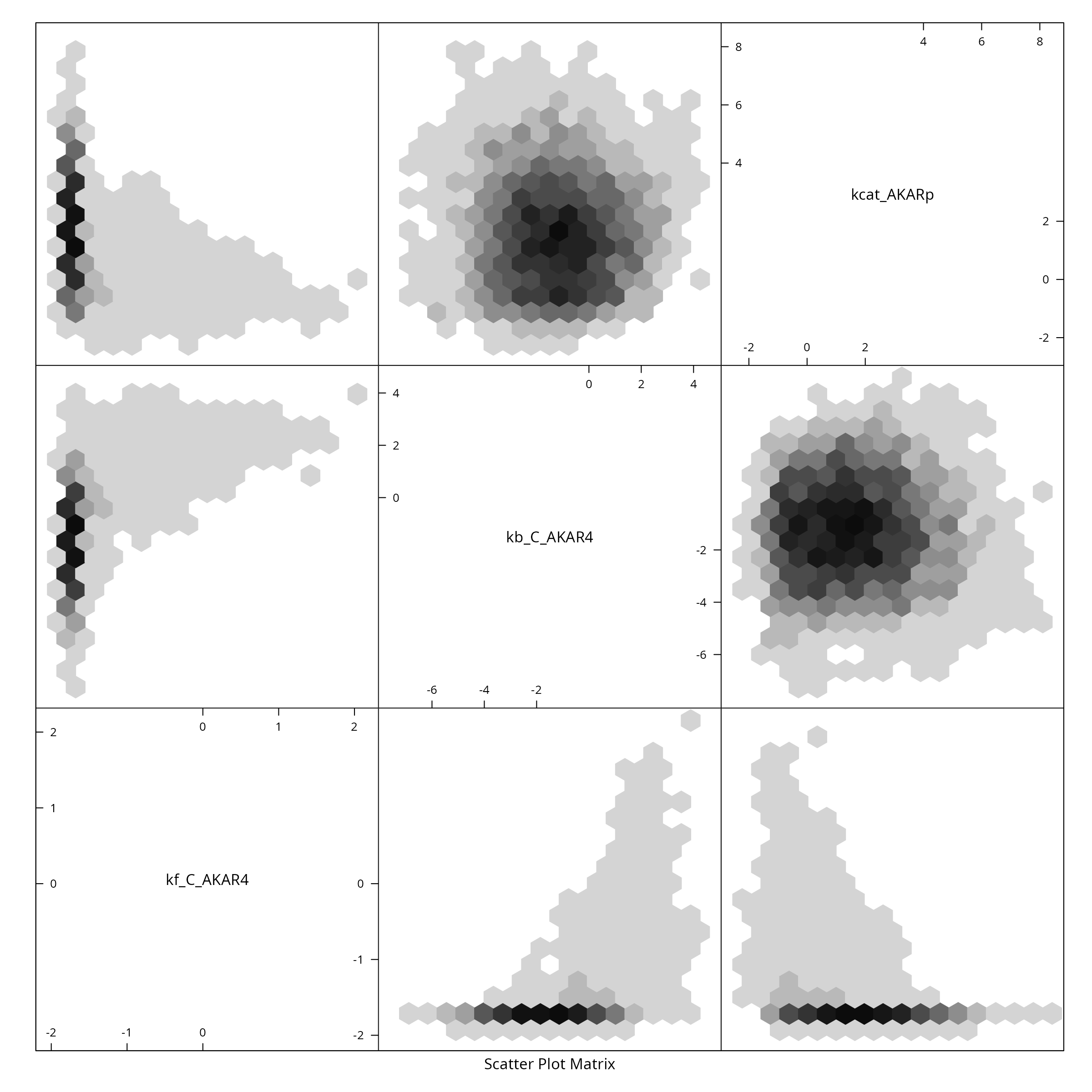
#> Effective sampple size: 6250

We reduce the sample for plotting purposes, by showing only every \(\tau_{\text{int.}}\)-th point and create a pairs plot for the first 6 parameters:

X <- Sample[seq(1,n,by=tau),]
colnames(X) <- rownames(sb$Parameter)
if (require(hexbin)){
    hexbin::hexplom(X,xbins=16)
} else {
    pairs(X)
}
#> Loading required package: hexbin