Sample AKAR4 via ABC • uqsa

library(uqsa)
library(parallel)
library(SBtabVFGEN)
library(rgsl)

We load the model from a collection of TSV files (inst/extdata/AKAR4 on github), the function below locates the tsv files after package installation:

modelFiles <- uqsa_example("AKAR4",full.names=TRUE)

Then we import the contents as a list of data.frames

SBtab <- sbtab_from_tsv(modelFiles) # SBtabVFGEN
#> [tsv] file[1] «AKAR4_100nM.tsv» belongs to Document «AKAR4»
#>  I'll take this as the Model Name.
#> AKAR4_100nM.tsv  AKAR4_25nM.tsv  AKAR4_400nM.tsv  AKAR4_Compound.tsv  AKAR4_Experiments.tsv  AKAR4_Output.tsv  AKAR4_Parameter.tsv  AKAR4_Reaction.tsv

We load the R functions of the model (e.g. the jacobian of the model):

AKAR4_vf, the vector field,
AKAR4_jac, the jacobian,
AKAR4_default, the default parameters

The R file we source additionally includes a variable called model, which serves the purpose of having generic names for all model constituents, to make it easier to write generic scripts:

model$vf() corresponds to AKAR4_vf()
- but does not use AKAR4 in the name
- otherwise identical
model$jac() corresponds to AKAR4_jac()
model$name is a string, "AKAR4" in this case

This can help to write fairly general scripts where the model’s name appears only at the top. You can investigate the sourced file to find out more.

Generally, model is a list of functions, one of which is called model$par() and returns the default parameters of the model in linear space:

source(uqsa_example("AKAR4",pat="^AKAR4[.]R$")) # loads "model"
model$name   # AKAR4

#> [1] "AKAR4"

model$par()  # default values for parameters

#> kf_C_AKAR4 kb_C_AKAR4 kcat_AKARp 
#>      0.018      0.106     10.200

model$init() # default initial values for ODE state variables

#>   AKAR4 AKAR4_C  AKAR4p       C 
#>     0.2     0.0     0.0     0.0

The model exists in R and C form: - AKAR4.R - AKAR4_gvf.c

The file ending in _gvf.c contains functions used for simulations with rgsl::r_gsl_odeiv2_outer() (_gvf.c needs to be compiled to a shared library). The functions in .R can be used more freely in R, and are functionally identical (they describe the same model, but solutions are slower in R).

The next function call checks that the model [...]_gvf.c file exist, and builds a shared library .so from these sources. It attaches a comment to its return value that indicates how the shared library for this model is named:

modelName <- checkModel("AKAR4",uqsa_example("AKAR4",pat="_gvf[.]c$")) # SBtabVFGEN
#> building a shared library from c source, and using GSL odeiv2 as backend (pkg-config is used here).
#> cc -shared -fPIC `pkg-config --cflags gsl` -o './AKAR4.so' '/home/andreikr/.local/R/library/uqsa/extdata/AKAR4/AKAR4_gvf.c' `pkg-config --libs gsl`
comment(modelName) # should be AKAR4.so
#> [1] "./AKAR4.so"

The comment will be used to find the .so file (if you move that file, adjust the comment on the modelName).

We want to sample in logarithmic space, so we set up a mapping function parMap. The sampler will call this function on the sampling variable parABC before it simulates the model.

parMap <- function (parABC=0) {
    return(10^parABC)
}

The ODE model receives a parameter vector p for each experiment. It consists of the biological model parameters (which are the same for all experiments), and input parameters (which together with initial conditions distinguish the experimental setups). This model doesn’t have input parameters, so the biological and ODE parameters are the same. Otherwise, two different kinds of parameters are concatenated into one big numeric vector inside of the solver. The model function AKAR4_default() returns the default values for p.

Next, we load the list of experiments from the same list of data.frames (SBtab content):

experiments <- sbtab.data(SBtab)
parVal <- AKAR4_default()
print(parVal)
#> kf_C_AKAR4 kb_C_AKAR4 kcat_AKARp 
#>      0.018      0.106     10.200

Define lower and upper limits for log-uniform prior distribution for the parameters:

ll <- log10(parVal) - 3
ul <- log10(parVal) + 3

Define Number of Samples for the pre-calibration npc and each ABC-MCMC chain ns. During ABC, we save every 100-th point, so work(nChains*ns*100) ≈ work(npc):

ns <- 2500  # ABC-MCMC sample size
npc <- 50000 # pre-calibration size

delta <- 0.02
set.seed(2022)
nCores <- parallel::detectCores()
options(mc.cores=nCores)

We define a function that measures the distance between experiment and simulation:

distanceMeasure <- function(funcSim, dataExpr, dataErr = 1.0){
  distance <- mean(((funcSim-dataExpr$AKAR4pOUT)/max(dataExpr$AKAR4pOUT))^2,na.rm=TRUE)
  return(distance)
}

If the data is very informative, then the difference between the prior and posterior are large. In such cases, it may be difficult to find the posterior through sampling. Dividing the data into chunks and processing them sequentially can help. Our model of the posterior of previous chunks is based on Copulas and the VineCopula package.

We divide the workload into chunks and loop over the chunks in th ecode block below.

The ABCMCMC function returns 1% of all sampled points, because of the very low acceptance rates of the ABC method. This is the reason for the comparatively low sample size request ns: the simulation workload will be proportional to 100*ns. But the returned sample is of a very high quality, with very low apparent auto-correlation (because we omitted the large number of repeated points).

chunks <- list(c(1,2),3)
priorPDF <- dUniformPrior(ll, ul)
rprior <- rUniformPrior(ll, ul)

start_time = Sys.time()
for (i in seq(length(chunks))){
    expInd <- chunks[[i]]
    simulate <- simulator.c(experiments[expInd],modelName,parMap,noise=TRUE)
    Obj <- makeObjective(experiments[expInd],modelName,distanceMeasure,parMap,simulate)
    time_pC <- Sys.time()

    pC <- preCalibration(Obj, npc, rprior, rep=3)
    time_pC <- difftime(Sys.time(),time_pC,units="secs")
    cat(sprintf("\t - time spent on precalibration: %g seconds\n",time_pC))

    time_ABC <- Sys.time()
    mcmc <- ABCMCMC(Obj, as.numeric(pC$startPar), ns, pC$Sigma, delta, priorPDF)
    time_ABC <- difftime(Sys.time(),time_ABC,units="mins")
    cat(sprintf("\t - time spent on ABC-MCMC: %g minutes\n",time_ABC))

    if (i>1){
        simulate <- simulator.c(experiments[chunks[[1]]],modelName,parMap)
        Obj <- makeObjective(experiments[chunks[[1]]],modelName,distanceMeasure,parMap,simulate)
        mcmc$draws <- checkFitWithPreviousExperiments(mcmc$draws, Obj, delta)
    }

    C <- fitCopula(mcmc$draws)
    priorPDF <- dCopulaPrior(C)
    rprior <- rCopulaPrior(C)
}

#> Warning in getMCMCPar(prePar, preDelta, p = p, sfactor = sfactor, delta = delta, : distances between experiment and simulation are too big; selecting the best (50000) parameter vectors.

#>   - time spent on precalibration: 49.4634 seconds
#> Started chain.
#> 
#> n = 10000
#> n = 20000
#> n = 30000
#> n = 40000
#> n = 50000
#> n = 60000
#> n = 70000
#> n = 80000
#> n = 90000
#> n = 1e+05
#> n = 110000
#> n = 120000
#> n = 130000
#> n = 140000
#> n = 150000
#> n = 160000
#> n = 170000
#> n = 180000
#> n = 190000
#> n = 2e+05
#> n = 210000
#> n = 220000
#> n = 230000
#> n = 240000
#> n = 250000    - time spent on ABC-MCMC: 59.7025 minutes

#> Warning in getMCMCPar(prePar, preDelta, p = p, sfactor = sfactor, delta = delta, : distances between experiment and simulation are too big; selecting the best (50000) parameter vectors.

#>   - time spent on precalibration: 30.7994 seconds
#> Started chain.
#> 
#> n = 10000
#> n = 20000
#> n = 30000
#> n = 40000
#> n = 50000
#> n = 60000
#> n = 70000
#> n = 80000
#> n = 90000
#> n = 1e+05
#> n = 110000
#> n = 120000
#> n = 130000
#> n = 140000
#> n = 150000
#> n = 160000
#> n = 170000
#> n = 180000
#> n = 190000
#> n = 2e+05
#> n = 210000
#> n = 220000
#> n = 230000
#> n = 240000
#> n = 250000    - time spent on ABC-MCMC: 30.539 minutes
#> 
#> -Checking fit with previous data
#> --  540  samples  did not fit previous datasets

end_time = Sys.time()
time_ = end_time - start_time
print(time_)

#> Time difference of 1.529996 hours

We plot the sample as a two dimensional histogram plot-matrix using the hexbin package:

colnames(mcmc$draws)<-names(parVal)
#
if (require(hadron)){
    ac <- hadron::uwerr(data=mcmc$scores,pl=TRUE)
    tau <- ceiling(ac$tauint+ac$dtauint)
    i <- seq(1,NROW(mcmc$draws),by=tau)
} else {
    i <- seq(1,NROW(mcmc$draws),by=100)
}


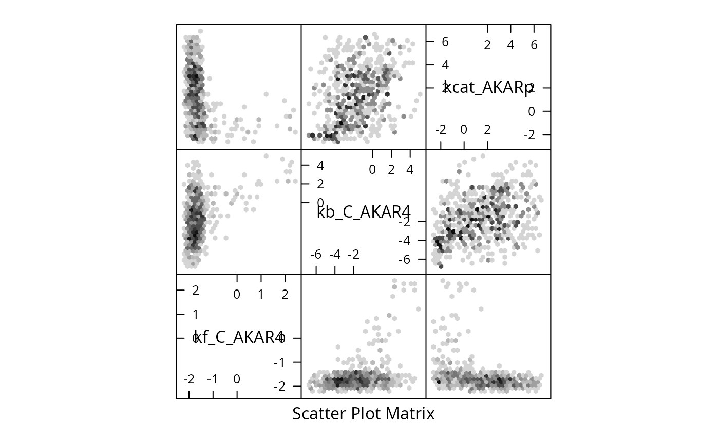
if (require(hexbin)){
    hexbin::hexplom(mcmc$draws[i,],xbins=10)
} else {
    pairs(mcmc$draws[i,])
}

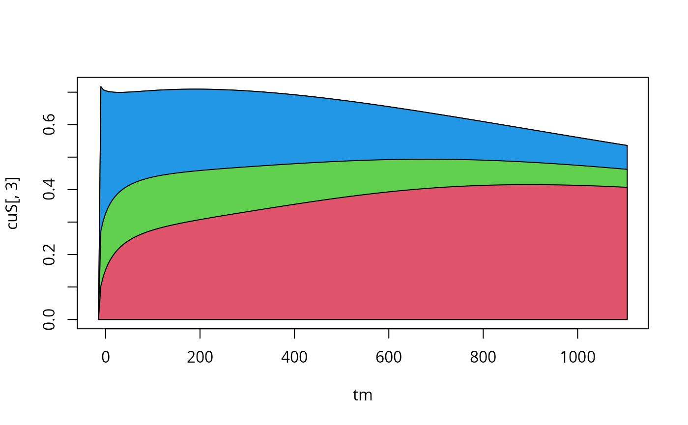
A sensitivity plot using the results of the above loop:

y<-simulate(t(mcmc$draws))
dim(y[[1]]$func)
#> [1]   1 225 756

where y[[1]] refers to the simulation corresponding to the first experiment: experiment[[1]], and $func refers to the output function values (rather than state variables). The outout functions are defined in the table SBtab$Output.

f<-aperm(y[[1]]$func[1,,]) # aperm makes the sample-index (3rd) the first index of f, default permutation
S<-globalSensitivity(mcmc$draws,f)
S[1,]<-0 # the first index of S is time, and initially sensitivity is 0
cuS<-t(apply(S,1,cumsum))
plot.new()
tm<-experiments[[3]]$outputTimes
plot(tm,cuS[,3],type="l",xlab="time",ylab="S",main="sensitivity (cumulative)")
## this section makes a little sensitivity plot:
for (si in dim(S)[2]:1){
    polygon(c(tm,rev(tm)),c(cuS[,si],numeric(length(tm))),col=si+1)
}